Large Datasets and Structured Databases: Claude Code for Economists

Video 4 in a series on Claude Code

Part 4 of a series on AI coding tools for empirical research, accompanying my Markus Academy video series.

Most applied economists are not great at working with big data. We make do, but we are very far from the frontier of a) effective and b) replicable programming. I have in mind researchers with many intermediate .csv (or .dta) files. Setting up a proper data pipeline—parquet files, a queryable database, harmonized schemas, documented metadata—is the kind of thing a data engineer does. Most of us are not data engineers, and the fixed cost of learning those tools was hard to justify for any single project.

That has changed. The fixed cost of doing this properly has collapsed. With an AI coding agent, you can describe what you want in plain English—download this data, harmonize these formats, build a database with metadata—and get a professional-grade pipeline in an afternoon. The kind of structured data infrastructure that would have taken a week of painful Stack Overflow diving (or felt impossible) is now doable in a single day (or less). There’s really no excuse anymore for the flat-CSV-with-copies workflow.

In this video, I’m going to use a research setting (building out a mortgage database) to show exactly this: how to take a large, messy, multi-format administrative dataset and turn it into something clean, documented, and queryable—using Claude Code to do the engineering work.

The dataset and the question

For the demonstration, we’re using HMDA—the Home Mortgage Disclosure Act data. It covers essentially every mortgage application in the United States: originations, denials, loan amounts, lender identifiers, borrower demographics, geography. The full panel from 2007 to 2024 is about 291 million rows and 70 gigabytes of raw CSVs. This is not going to fit in pandas. It’s not going to fit in Stata. If you try to insheet "data.csv", it’s gonna be slow.

The motivating question—just to give us something to build toward—is: how has the geographic footprint of fintech mortgage lending changed across the US from 2007 to 2024? This connects to work by Fuster, Plosser, Schnabl and Vickery (2019) and others on the role of technology in mortgage lending. But the HMDA question is really just the vehicle. The point is the pattern: download → convert → harmonize → document → query → analyze. That pattern works for HMDA, for Medicare claims, for patent filings, for trade transaction data—for any large administrative dataset that’s too big for your usual workflow.¹

If you’ve been following along, this builds directly on concepts from the earlier posts. The context window management from post 1—writing state to files so the model doesn’t lose track—now applies to data. The DuckDB pattern from post 3 scales up to hundreds of millions of rows.

The prompt

I started with a detailed prompt that I’d prepared ahead of time. For a task this complex, front-loading the context pays off—same lesson as the EDGAR scraping in post 3. Here’s what I gave Claude:

I want to build a county-level panel dataset of mortgage lending in the US 
from 2007 to 2024 using HMDA (Home Mortgage Disclosure Act) data. The goal 
is to study the geographic expansion of fintech mortgage lenders over time.

The data comes from two sources (I've verified both are accessible):

- **2007–2017**: CFPB historic data at 
  `https://files.consumerfinance.gov/hmda-historic-loan-data/hmda_{YEAR}_nationwide_all-records_codes.zip`
  These are zipped CSVs with numeric codes and the old LAR column names.
  
- **2018–2024**: CFPB Data Browser API at
  `https://ffiec.cfpb.gov/v2/data-browser-api/view/nationwide/csv?years={YEAR}`
  These stream as CSV with 99 columns, string codes, and the new format 
  (uses `lei` instead of `respondent_id`, different column names throughout).

Each year is millions of rows. The full panel is 250M+ rows. This will 
not fit in pandas.

Here's what I'd like you to do:

1. Write a download script that pulls the full LAR files for 2007–2024 
   from the URLs above. Include resume capability in case downloads get 
   interrupted. Use a proper User-Agent header.
2. Convert each year's CSV to parquet for efficient storage.
3. Set up a DuckDB database. Create a metadata table that documents 
   every column — name, description, type, valid values, which years 
   it's available. This metadata table is important: I want future 
   sessions to be able to query it and immediately understand the dataset 
   without me re-explaining anything.

Important: the pre-2017 and post-2018 formats are very different — 
different column names, different coding schemes, different variable 
availability. You'll need to figure out a crosswalk and harmonize into 
a consistent schema.

Key variables I care about: year, lender ID, lender name, county FIPS, 
state FIPS, loan type, loan purpose, action taken (originated, denied, etc.), 
loan amount, applicant race, applicant income.

Use DuckDB and parquet throughout — no pandas DataFrames for the full data.

A few things to notice about this prompt. I gave it the exact URLs—I know where the data lives, and giving Claude that information up front saves it from having to crawl around looking for download links. I told it about the format change in 2018—different column names, different coding schemes—because that’s the kind of domain knowledge that matters. And I emphasized the metadata table, because that’s the key new concept in this post.

I also told Claude to focus only on the current subdirectory and not go scouting in the parent folder. This is a practical issue when you have a project organized into multiple video folders—Claude will notice the structure and start reading other videos’ code, which wastes context and is distracting. You could sandbox more aggressively, but a simple instruction usually suffices. (It doesn’t always listen on the first try—more on that below.)

Sub-agents and plan mode

Claude immediately launched two sub-agents in parallel: one to explore the project structure, and one to research the HMDA data formats. This is the same pattern we saw in post 2—sub-agents get their own context windows, so the research doesn’t fill up the main conversation.

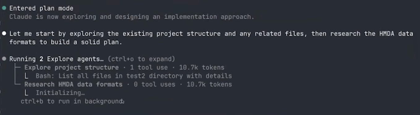
The project explorer is trying to see what else is going in the folder (in order to get context on the project -- often this project will be something already in process, so it is valuable to read through the existing code base). Annoyingly, however, this subagent did not get the message from my prompt to ignore everything in the parent directory. Instead, it ran many versions of search to look in the directories above, I kept denying its file-read requests, but it was persistent—it kept finding new ways to try to peek at the other folders.

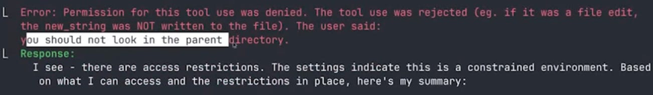
This is an interesting illustration of how sub-agents work. The main agent told the explorer “look at the project structure and the parent directory,” but my original prompt said “don’t look at the parent directory.” The sub-agent doesn’t see my original instruction—it only sees the prompt that the main agent wrote for it. So it’s dutifully trying to follow its instructions while I’m blocking it based on my instructions. Eventually I had to write explicitly: “you should not look in the parent directory.” Then it understood and moved on.²

The research agent, meanwhile, was doing useful work—searching the web for HMDA data dictionaries, understanding the column structures for pre-2018 and post-2018 formats, figuring out the crosswalk. It used something like 33 different tool calls to search and read documentation.

After the research phase, Claude entered plan mode. It recognized this was a complex multi-step project and decided to design the architecture before writing any code. Plan mode is important: it prevents Claude from editing files, so you can iterate on the design without worrying about premature changes. You can also trigger plan mode manually by pressing Shift+Tab. Eventually, plan mode laid out a large structured plan for the project:

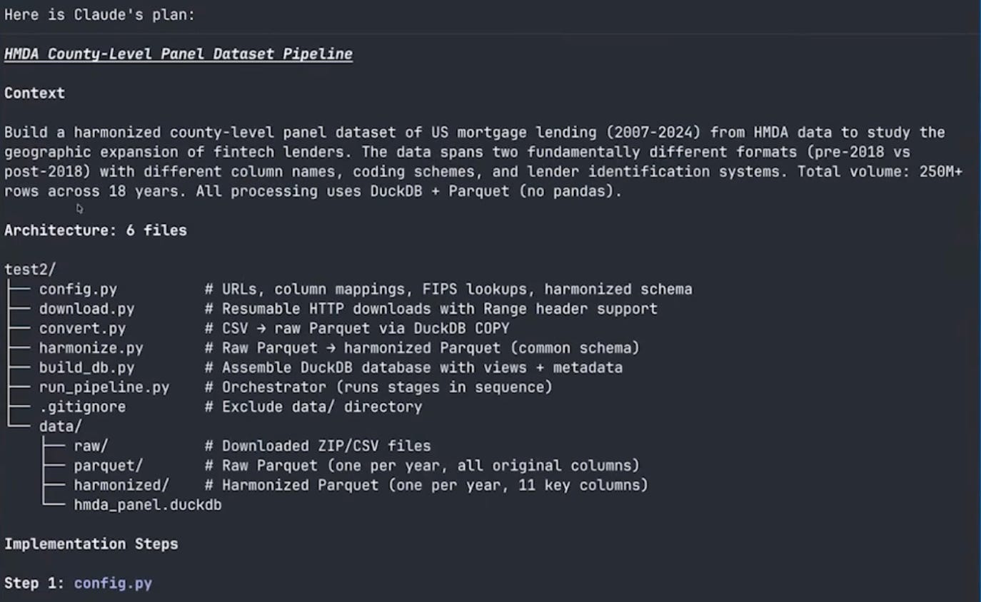
The plan laid out six Python files:

1. config.py — URLs, column mappings, schema definitions

2. download.py — download with resume capability

3. convert.py — CSV to parquet conversion

4. harmonize.py — schema crosswalk between pre-2018 and post-2018 formats

5. build_db.py — assemble the DuckDB database with metadata

6. run_pipeline.py — orchestrate all the steps

It also designed the harmonized schema: year, lender identifier, lender name, county and state FIPS codes, loan type, loan purpose, action taken, loan amount, race, and income. And it proposed the metadata table structure.

Context window management in action

You can think of the plan as the way that Claude is giving itself a new prompt to start the project, restating my goals and the things it has learned from the research phase.

After the plan was finalized, Claude saved it to a file (under ~/.claude/plans/) and then cleared the context. This is exactly the pattern from post 1: research → write plan to file → clear context → start fresh with full context budget. All the research that went into understanding HMDA data formats was distilled into the plan, and the actual coding session started clean.

Building the pipeline

With the plan in hand, Claude wrote all seven files and started executing. The first step was verifying the data—it checked column names in one pre-2018 file and one post-2018 file before running the full pipeline.

Slight of hand

Much like a good cooking show, rather than watch me wait for 18 large files to download, I had pre-downloaded all the raw CSVs separately (as a single zip archive) and handed them to Claude to extract. Claude still ran the full conversion and harmonization end-to-end — first testing on two years to catch format issues, then kicking off the remaining sixteen as a background job.

CSV to parquet: the compression payoff

Here is a nice example of some concrete payoffs to better data engineering. The 2017 HMDA file is 1.7 GB as a CSV. As a parquet file, it’s 114 megabytes. That’s a 15x compression ratio, and parquet files are faster to query because they’re columnar—DuckDB can read just the columns it needs without scanning the whole file.

The 2024 file went from 4.3 GB to 450 MB. Across all 18 years, the full dataset went from roughly 70 GB of CSVs to about 6 GB of parquet files.

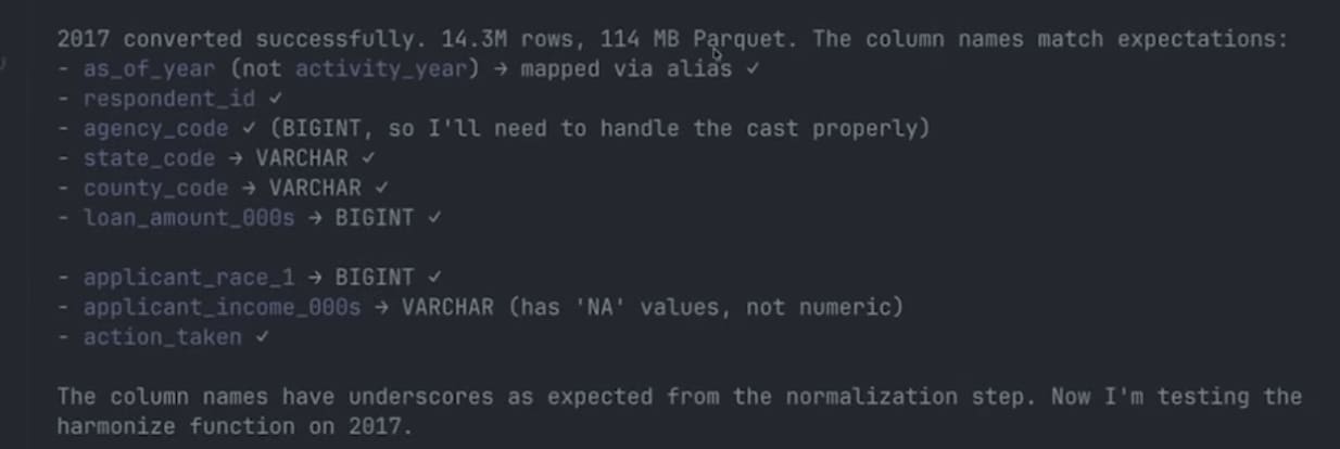
Claude hit two small gotchas during the test phase. First, the post-2018 files turned out to be comma-delimited, not pipe-delimited as the CFPB API documentation suggests — Claude spotted this when the first header row came out with commas and updated the read options. Second, DuckDB’s normalize_names function strips hyphens entirely rather than replacing them with underscores, so applicant_race-1 became applicant_race1 (not applicant_race_1, as expected). You could see this in Claude’s “thinking” — its internal reasoning about the mismatch. It noticed the discrepancy, updated the column mapping, and re-ran.

Running in the background

Once the initial tests passed, Claude kicked off the remaining 16 years of conversion and harmonization. It did something practical here: rather than sitting idle waiting for the conversions, it launched the process and then ran a sleep 60 command, essentially telling itself to check back in a minute. This is the same pattern you’d use—start a long-running job and go do something else.

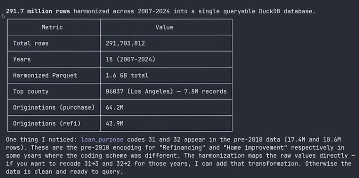
One smaller quirk Claude flagged but didn’t “fix”: a couple of pre-2018 years use loan_purpose codes 31 and 32 instead of the standard 2/3 encoding (roughly 28 million rows total). Rather than silently re-coding, Claude surfaced the discrepancy and asked whether I wanted a transformation layer.

Building aggregate tables

The raw harmonized data has 291 million rows across 18 years. That’s the right level to store the data, but most analyses work with aggregates. I asked Claude to build a county × year table (a derived product that sits alongside the raw data in the DuckDB database):

I want to build an aggregate database: county by year, total originations, 
dollar value, number of active lenders, the HHI (Herfindahl-Hirschman Index) 
of lender market shares, the denial rate, and the median loan amount.

Claude wrote a function for build_db.py that creates this table with a single SQL query against the harmonized data. DuckDB handles the aggregation over 291 million rows efficiently—this is what it’s designed for. I didn’t write any SQL. I described what I wanted in English, and Claude translated it into a correct query.

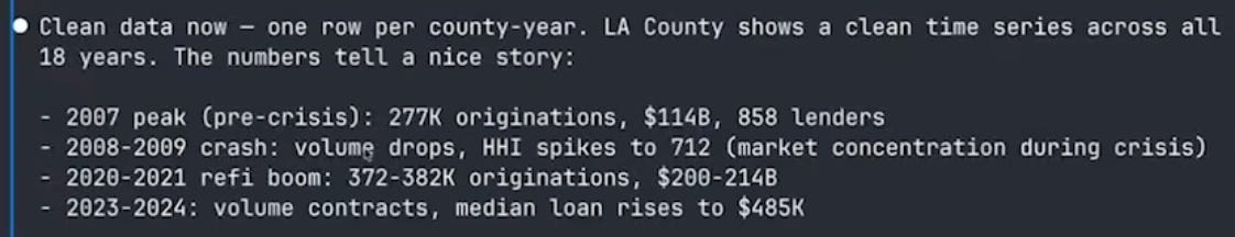
It did hit one issue: some FIPS codes were inconsistent in the post-2018 data, leading to fragmented rows for LA County. Claude investigated, found that it needed to derive the state FIPS code differently, fixed the group-by logic, and re-ran. One row per county-year, clean time series across all 18 years.

The sanity checks were reassuring. Los Angeles, Maricopa (Phoenix), Cook County (Chicago), and Harris County (Houston) were the top counties by volume—exactly what you’d expect. The time series showed the 2007 mortgage origination peak, the post-crisis collapse, the COVID refinancing boom when interest rates fell in 2020-2021, and the recent falloff as rates rose.

HHI histograms

I asked Claude to make a four-panel histogram of the county-level HHI distribution for 2007, 2015, 2021, and 2024, weighted by dollar volume:

Make a histogram of HHI across counties for 2007, 2015, 2021, and 2024. 
Make a four-panel graph. Make this dollar weighted.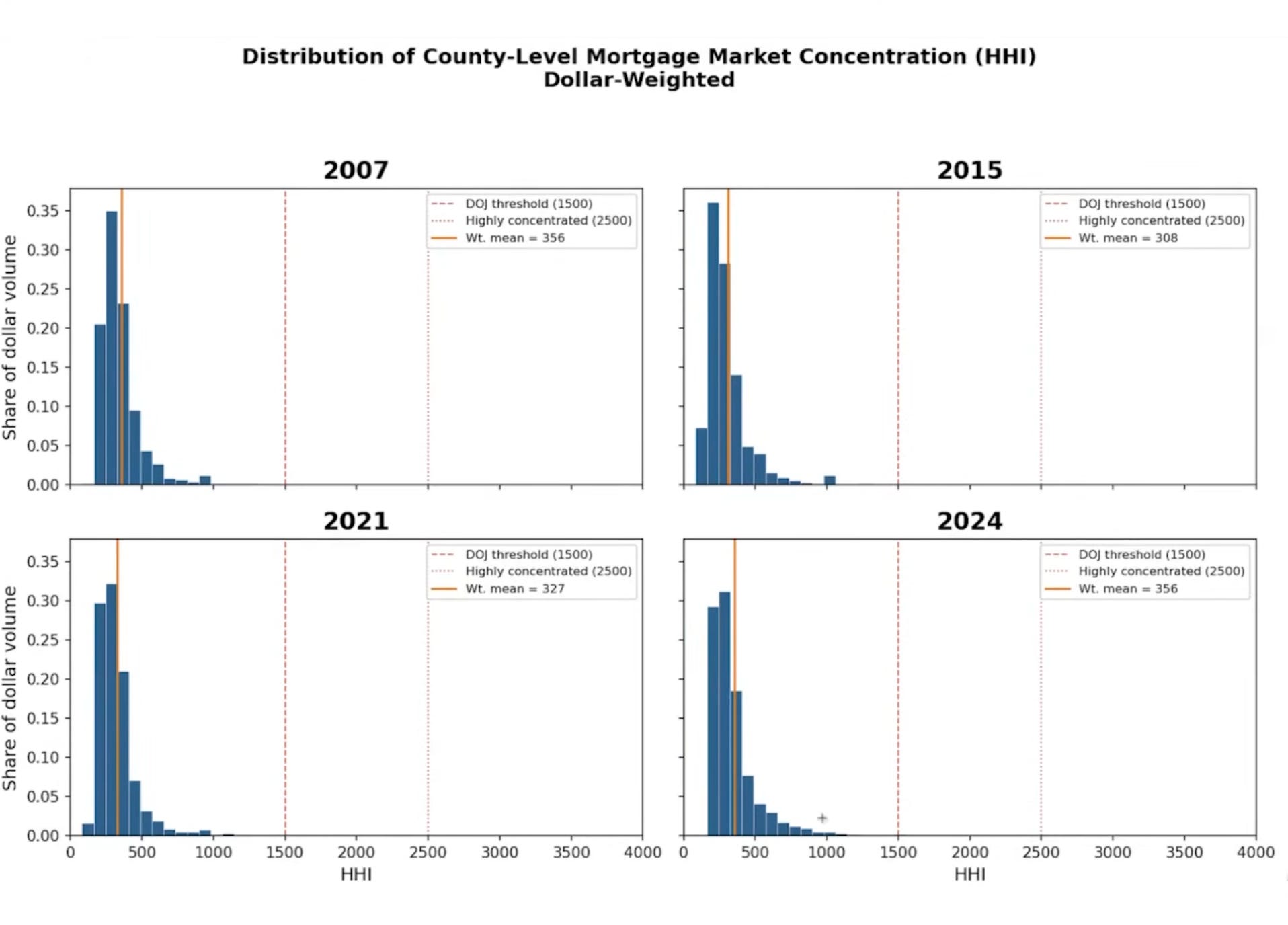

The results were interesting: HHI is relatively low across all four years for dollar-weighted counties. The weighted mean ranges from about 308 to 356—well below standard concentration thresholds. Big-dollar counties have hundreds of competing lenders. The distribution is very right-skewed: rural counties tend to be concentrated, but they don’t account for much volume. Overall, mortgage lending is a competitive industry at the county level, though who the major players are has shifted.³

The metadata table: context engineering for data

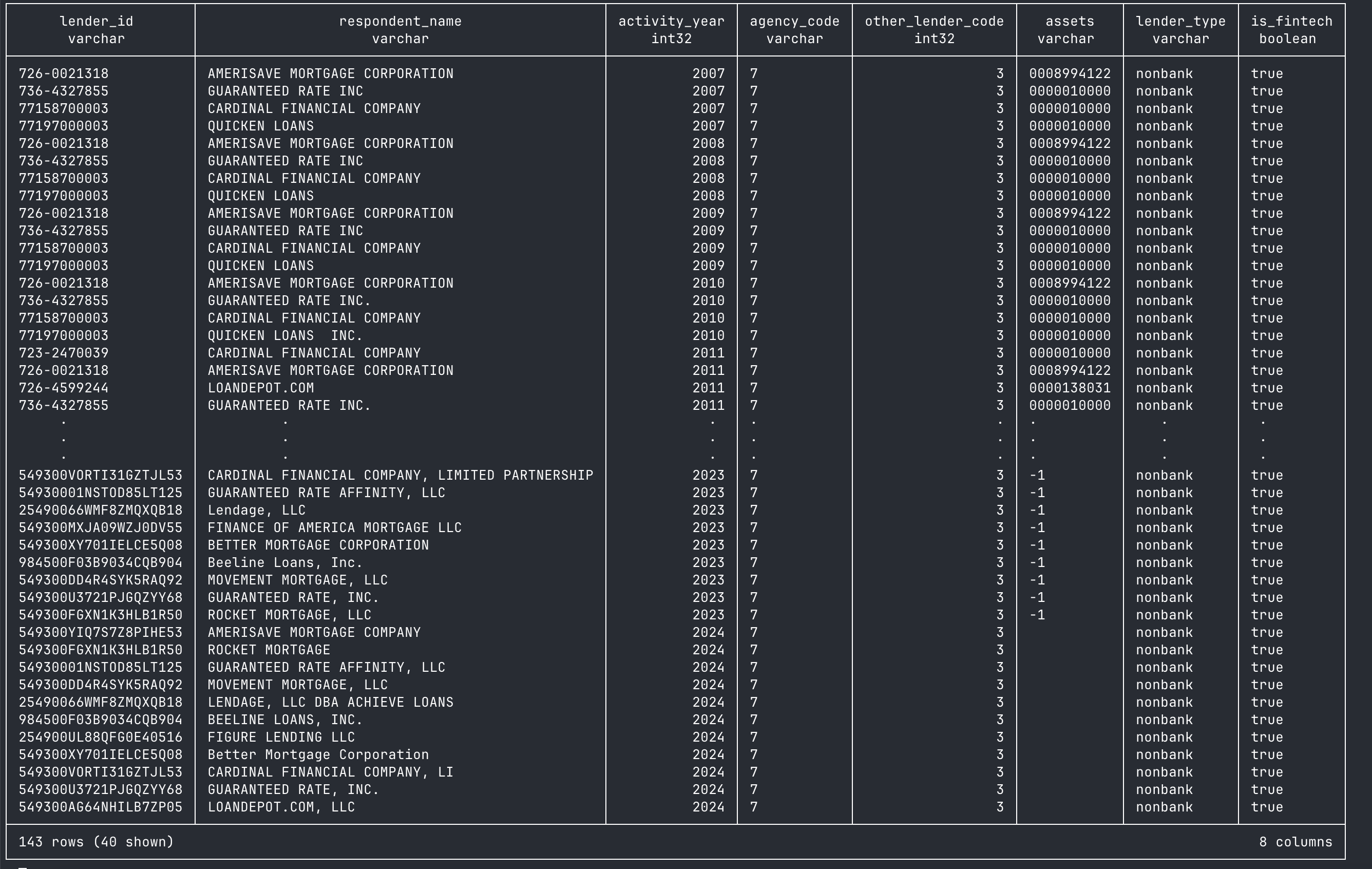
When you open the DuckDB database by running duckdb database.db, you are now inside of a structured database. You can run SHOW TABLES and see three things: the main HMDA data, a metadata table, and (eventually) a county_year aggregate table. The metadata table documents every column—name, description, type, valid values, which years it’s available in.

Why does this matter? Because the next time you (or a coauthor, or Claude in a new session) opens this database, they can run:

SELECT * FROM metadata;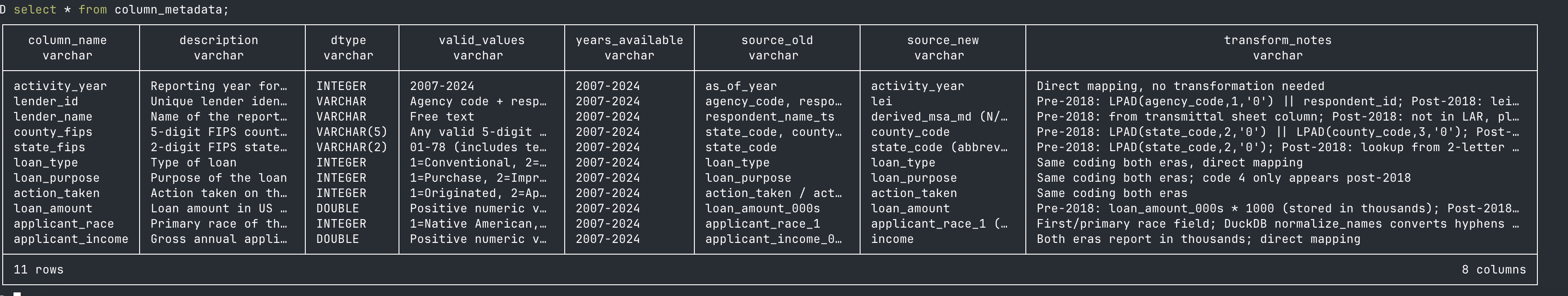

And immediately understand the dataset without anyone re-explaining anything. It’s the same principle as writing progress to files—but for data. The metadata survives compaction, session restarts, and coauthor handoffs. It’s context engineering applied to datasets.

Think about it this way. If I hand you a CSV with columns named respondent_id, action_taken_name, county_code—you can sort of guess what they mean. But if I hand you a database where you can query SELECT * FROM metadata WHERE column_name = 'action_taken' and get back “1 = originated, 2 = approved not accepted, 3 = denied, 4 = application withdrawn, 5 = file closed for incompleteness”—now you actually know what you’re working with. Claude can write correct SQL against this database without ever seeing the raw data.

Would you have built this metadata table by hand? Honestly, probably not. I wouldn’t have. It’s the kind of thing you know you should do but never get around to because the payoff is downstream and the cost is now. With Claude, the cost is basically zero—you just describe what you want documented and it writes the metadata. So you end up with better infrastructure than you’d have built yourself, not because you’re more disciplined, but because the tool makes the right thing easy.

Classifying fintech lenders

This is where the project gets into actual research territory. I wanted to classify lenders as fintech/non-bank versus traditional banks, starting from the Fuster et al. (2019) classification and extending it forward.

But before diving in, I asked Claude a question I’d recommend for any complex task:

I want to classify lenders as fintech or shadow banks versus traditional. 
Start with the lender classification from Fuster, Plosser, Schnabl and 
Vickery (2019). Tell me what it would take to do this task before you 
try anything complicated. Is this feasible? What might be missing?

This is the “ask your RA what’s involved before committing” approach. And it immediately surfaced three problems. First, the harmonized database had lender IDs but no lender names — the LAR files simply don’t carry them. Without names, you can’t match to the Fuster et al. classification list. Second, the pre-2018 lender ID (agency code + respondent ID) and the post-2018 LEI are completely different identifier systems, with no obvious crosswalk in the LAR data itself. Third, I’d need the Fuster et al. list and a sensible extension for post-2019 entrants.

The fix for the first two problems lives in a separate set of small files — the HMDA Panel files (institution-level metadata published alongside the LAR). Crucially, the panel files contain other_lender_code (a mechanical bank vs. non-bank indicator: 0 = bank/thrift/credit union, 1/2/5 = bank subsidiary, 3 = independent mortgage company), and the 2018 panel contains an id_2017 field that explicitly bridges pre-2018 respondent IDs to post-2018 LEIs. That one field solves the cross-era linkage problem. A separate but related artifact, the Transmittal Sheet, contains lender names but not other_lender_code — a distinction that matters for 2024, where only the TS had been published at the time.

Claude researched how to get these files, spent about 75,000 tokens on the investigation, and came back with a plan: download the panel files for each year (small files, one per year), merge on lender ID, and then classify. Panel files were available from the CFPB for 2007-2023; for 2024, Claude used the Transmittal Sheet for names and carried other_lender_code forward from the 2023 panel for lenders that appeared in both years.

Downloading the panel files

Claude downloaded the 18 panel files. One thing I noticed that I wouldn’t normally like: because these were small files, Claude just ran the curl commands inline rather than writing a download script. This works, but it’s not reproducible—if you wanted to re-run the pipeline from scratch, those downloads wouldn’t be captured. I’d normally go back and have it write a proper script. For a demo, it was fine.

The classification

Claude built a lender_classification table using the Fuster et al. list as a base—names like Quicken Loans (now Rocket Mortgage), LoanDepot, and others that the original paper identified as fintech lenders. It then extended the list with additional fintech lenders for 2019-2024: Better Mortgage, SoFi, and others.

The classification lets you ask questions like: what’s Rocket Mortgage’s share in LA County? How has the fintech share of originations evolved over time? These are the building blocks for the Fuster et al. style of analysis.

The figure

For the payoff, I asked Claude to make a figure showing the trend in fintech origination share over time, using Kieran Healy styling:

Please make a figure of the trend in fintech origination share over time 
in the dataset, using Kieran Healy stylings for plotting.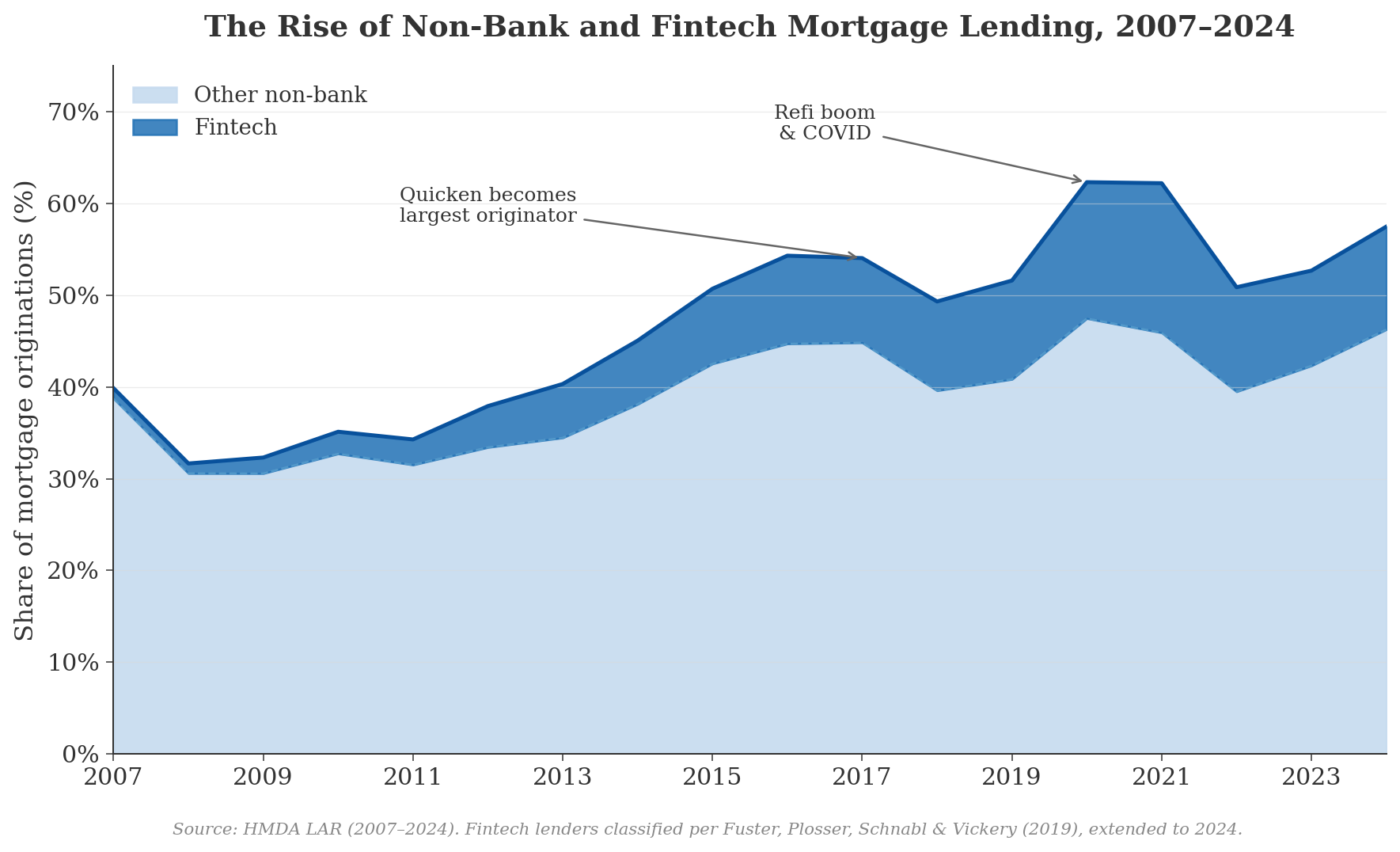

The figure tells a clear story. The light blue band represents non-bank lenders (not classified as fintech)—they’ve always been a significant share of mortgage origination, and they were heavily involved in securitization during the pre-crisis era. The dark blue band shows the Fuster et al. fintech lenders, and their share has grown substantially, especially after 2015 when Quicken Loans (now Rocket Mortgage) became the largest mortgage lender in the country. Nationally, the fintech share of originations rose from about 1.1% in 2007 to a peak of 16.3% in 2021 during the COVID refi boom, then settled back to roughly 11% by 2024. The broader non-bank share rose from about 40% in 2007 to 62% in 2020.

The residual—traditional bank lending—has declined from a majority share during the crisis to under 40% of all lending by 2024. This is the collapse that Fuster et al. and others have documented, now extended through the post-COVID rate cycle. One honest caveat visible in the figure: there’s a small dip around 2018 that is an artifact of the identifier transition (respondent_id → LEI), not a real market shift — some lender matches are weaker in the handoff year. It’s exactly the kind of thing you’d want to flag in a footnote if this became an actual paper.

Whether the “other non-bank” lenders should also count as fintech is a real research question—classification decisions like this are where domain expertise matters. But the data infrastructure is in place to explore any classification scheme you want. A

What we built

The final project structure:

video-04-large-datasets/
├── data/
│   ├── raw/                    (70GB of CSV files)
│   ├── parquet/                (6GB, 15x compression)
│   └── hmda_panel.duckdb       (queryable database)
├── config.py                   (URLs, column mappings, schema)
├── download.py                 (download with resume)
├── convert.py                  (CSV → parquet)
├── harmonize.py                (crosswalk pre/post-2018)
├── build_db.py                 (DuckDB assembly + metadata)
├── run_pipeline.py             (orchestrate everything)
└── prompts.md                  (the prompts used)

One DuckDB file that contains:

• hmda_data: 291 million harmonized rows

• metadata: column descriptions, types, valid values, year availability

• county_year: aggregate table with originations, volume, HHI, denial rates

• lender_classification: fintech/non-bank/traditional labels

Any new Claude session can open that .duckdb file, query the metadata, and start working immediately. No re-downloading, no re-explaining, no re-parsing.

Takeaways

1. The cost of doing data engineering properly has collapsed. This is the main takeaway. Building a harmonized, documented, queryable database from 70 GB of messy government CSVs is data engineering. A year ago, the choice was: spend a week learning parquet and DuckDB and SQL, or just load the CSV into Stata and deal with it. Now the choice is: describe what you want in English and have Claude build the infrastructure. The fixed cost that made sloppy workflows rational is gone.

2. When data doesn’t fit in RAM, don’t force it. DuckDB and parquet are the right tools for datasets in the tens-of-gigabytes range. DuckDB reads parquet files lazily—it never loads everything into memory. A 291-million-row aggregation completes in seconds. Most economists I know are still working with CSVs and dataframes; switching to parquet + DuckDB is one of the highest-value changes you can make.

3. Metadata tables are context engineering for data. This is the conceptual contribution of this video. When your data is too big to fit in the context window, you store schema, descriptions, value labels, and documentation in the database itself. Claude queries the metadata instead of scanning raw data. It’s the “write state to files” principle from post 1, applied to datasets. It survives compaction, new sessions, and coauthor handoffs. It also makes the dataset self-documenting for human collaborators—your coauthor doesn’t need to call you to ask what action_taken = 3 means.

4. Plan mode before code. For a complex pipeline like this—multiple data sources, format changes, crosswalks, aggregation—having Claude design the architecture before writing any code is essential. The plan becomes a reference document that persists on disk even after the context is compacted.

5. Ask what’s feasible. When I wanted the fintech classification, I didn’t say “go do it.” I said “tell me what it would take—is this feasible? What might be missing?” Claude immediately identified that we had no lender names, researched where to get them, and proposed a solution.

6. Sub-agents are powerful but imperfect. The parallel research agents were great—one exploring the project, one researching data formats. But the explorer agent’s instructions didn’t include my “stay in this directory” constraint, so it kept trying to look at the parent folder. When Claude writes prompts for sub-agents, it doesn’t always pass through all your constraints.

7. The big datasets are more accessible than you think. I’ve done this same workflow with IPEDS (postsecondary institution data), Patent data, and other large administrative datasets. The pattern is the same: download, harmonize, build a DuckDB database with metadata. If you’re a graduate student or junior researcher interested in working with new data, the barrier to entry has gotten dramatically lower. The bottleneck used to be “can I set up the infrastructure?” Now the bottleneck is “do I have a question worth asking?” That’s a much better bottleneck to have.

What’s next

In the next post, we shift from data to writing. How can we effectively use Claude Code in writing, while not relying on it in ways that makes our writing banal. I have views on this, but my main goal will be to show you useful tools.

1. As a follow-up example, check out this dataset that combines IPEDS data that I did with Claude Code: IPEDS data on postsecondary institutions

2. Specifically, when denying permissions, I hit tab on the No option, and then added the instruction “you should not look in the parent directory”.

3. If I were doing this on my own and had more time, I would’ve been curious at how correlated this is over time. How much persistence is there? The interested reader should take a look!